LUT programming

LUT are instanced in SDP/CDP in NVDLA, it’s used to mimic the non-linear functions (Sigmoid/TanH/LRN, etc.) of a network. As we know, the LUT precision is highly depends on LUT entries and slope variation of the curve: The more LUT entries, the higher precision. On the other hand, the strong slope variation of the curve, the hard to mimic.

It’s worth to mention SDP/CDP shares the same LUT logic, the only difference between them are the bit-depth as SDP pipeline is 32bits but CDP pipeline is 37bits.

We proposed an innovated 2 level hybrid LUT architecture to keep very high precision by limited LUT entries:

There’re 2 highlights of this implementation:

• 2 level:

Fig. 32 LUT architecture

There’re 2 tables (X/Y table), the typical configuration is use one of them as raw table to cover entire dynamic range and the other work as density table to cover a small portion of the dynamic range. Due to the coverage difference, raw table has low sample rate but density table has relative high sample rate, this is inspired by the attribute of LRN/Sigmoid/TanH curve:

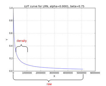
Fig. 33 Non-linear function: LRN

Fig. 34 Non-linear function: Sigmoid

We can see from figures above, for those functions, only a small portion has significant slope variation and the others portion almost without too much change thus 2 level LUT is an economy option to mimic those functions.

As there might be overlap between density/raw table, we have a programmable register: “priority” (pri) to allow software control which LUT table output should be taken as final output when one sample fits to both tables. Of course, the suggestion is to use density output all the time.

• Hybrid working mode

We noticed for LRN, the input dynamic range is very high (0~10^8), but most of the samples are within a small data range:

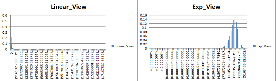
Fig. 35 Histogram of LRN LUT input

Histogram above are collected from “pool1/norm1” layer of GoogleNet, we viewed the same data by different x-axis coordinate system (linear and exponential).

We can see the linear view merges >50% samples to one point in histogram while exponential view distinguishes those samples to different histogram points which gives much better resolution. Same strategy can be adopted to LUT: If the LUT is working on exponential mode, we have a very high sample rate on low range values and low sample rate on high range values (it’s fair since they have low frequency in histogram). This is the idea of “exponential” mode. Currently, only X table is able to work on exponential mode and when this mode is enabled, the coverage is fixed as \(2^{exp\_start} ~ 2^{exp\_start + tlb\_entry}\)

Table below summarized the LUT attributes of NVDLA (The X/Y are used to denote different table, when mapping to hardware, X corresponding to LE(Linear/Exponent) while Y corresponding to LO(Linear only)):

Attributes	Description
X table entries	65
Y table entries	257
Bits per entry	16
X supported working modes	Exponential/Linear
Y supported working modes	Linear
Interpolation methods	Linear interpolation
Out-of-range behavior	Linear interpolation

Recommended LUT configuration for typical use scenarios:

Use scenario	Configuration
LRN	X – Exponential mode (worked as raw table) Y – Linear mode (worked as density table)
Activation (Sigmoid/TanH, etc.)	X – Linear mode (worked as density table) Y – Linear mode (worked as raw table)

However, this is not mandatory, software can program LUT work as any of cases below (X/Y can be reversed, which means totally 6 cases):

Fig. 36 LUT coverage

As shown in Fig. 32, there’re couple parameters for LUT, let’s discuss how to configure them based on different modes.

Exponential mode

If LUT is working on exponential mode and LUT storage has example below (actually, exp_start is programmable):

exp_start=-32 LUT[0]=f(2exp_start)=f(2-32) LUT[1]=f(2exp_start+1)=f(2-31) … LUT[64]= f(2exp_start+64)=f(232)

Suppose LUT input is: \(x' = (x - O_{in}) * SF_{in}\), per LUT storage, the index should be:

\[index = (log_2(x - linear\_start)) - exp\_start = log_2 (\frac{x'}{SF_{in}} + O_{in} - linear\_start) - exp\_start\]

SF_in must be 2^M, then, formula above changed as: .. math:: index = log_2 (frac{x’}{SF_{in}} + O_{in} - linear_start) - exp_start = log_2 (x’ - SF_{in}(linear_start - O_{in})) - (M + exp_start)

exp_start is a value related to LUT storage (in our example, we use -32 here) while M is related to upstream convertor setting.

The mapping between register and symbols above are lists below (only X table supports exponential mode):

Register	Symbol
LE_INDEX_OFFSET	M+exp_start
LUT_LE_INDEX_SELECT	Not used
S_LUT_LE_START_LOW/HIGH	\(SF_{in}(linear\_start - O_{in})\)

Linear mode

If LUT is working on linear mode and LUT is supposed to cover min~max, then, LUT entry storage should be (suppose entry_num=257):

step=(max-min)/(entry_num-1) LUT[0]=f(0*step + min) LUT[1]=f(1*step + min) … LUT[256]=f(256*step + min)=f(max)

Suppose LUT input is: \(x' = (x - O_{in}) * SF_{in}\), per LUT storage, the index should be:

\[index=\frac{x-min}{step}=\frac{\frac{x'}{SF_{in}}+O_{in}-min}{step}=\frac{x'+O{in}*SF_{in}-min*SF_{in}}{(max-min)*SF_{in}}*(entry\_num-1)\]

Denote:

\[SF_{lut}=\frac{entry_num-1}{(max-min)*SF_{in}},\ O_{lut}=min*SF_{in}-O_{in}*SF_{in},\ index=(x'-O_{lut})*SF_{lut}\]

This requires multiplier, in order to make hardware simpler, we require:

\[SF_{lut} = 2^M\]

Then, hardware just need to right/left shifter to get correct index, however, this implies:

\[(max - min) * SF_{in} = 2^{C-M}, where\ C=log_2(entry\_num - 1)\]

This can be guaranteed by the convertor before LUT (cdp_in_cvt in CDP; X/X/Y multiplier in SDP).

The mapping between symbols above and the actual registers are (X could be LE/LO):

Register	Symbol
LUT_LE/LO_INDEX_SELECT	-M
X_START_LOW/HIGH	\(O_{lut}\)
LE_INDEX_OFFSET	Not used

Out-of-range control

Suppose one LUT has coverage between [min, max]. If one input sample bigger than max or smaller than min, we call it out-of-range sample.

NVDLA supports linear interpolation of those out-of-range samples. The mathematic formula for the interpolation is (x is the input sample value):

\[\begin{split}\begin{equation}\begin{cases} y_0+(x-min)*k_{underflow},&\text{x<min}\\ y_n+(x-max)*k_{overflow},&\text{x>max}\\ \end{cases}\end{equation}\end{split}\]

From hardware perspective, the interpolation is:

\[\begin{split}\begin{equation}\begin{cases} LUT[0]+(X-START)*UFLOW_{SCALE}/UFLOW_{SHIFT},&\text{X<START}\\ LUT[N]+(X-END)*OFLOW_{SCALE}/OFLOW_{SHIFT},&\text{X>END}\\ \end{cases}\end{equation}\end{split}\]

Take underflow as an example, given (\(2^M\) is the scaling applied on LUT input, SF is the scaling applied on LUT entries):

\[X = x * 2^M\]

\[START = min * 2^M\]

\[LUT[0] = y_0 * SF\]

Hardware output:

\[\begin{split}\begin{align*} LUT[0] + (X-START)*UFLOW\_SCALE/UFLOW\_SHIFT & = y_0 * SF + (x-min) * 2^M * UFLOW\_SCALE/UFLOW\_SHIFT \\ & = SF*(y_0 + \frac{(x-min) * 2^M * UFLOW\_SCALE/UFLOW\_SHIFT}{SF}) \end{align*}\end{split}\]

Thus:

\[\frac{2^M * UFLOW\_SCALE/UFLOW\_SHIFT}{SF} = k_{underflow}\]

The mapping between the symbols in above formula and registers are:

Register	Symbol	NOTE
LUT[0]	\(y_0\)	No register, directly use LUT content
LUT[N], (N is the last entry of the LUT)	\(y_n\)	No register, directly use LUT content
X_START_LOW/HIGH	Min*2M	Same bits/encoding as the pipeline. (i.e.: for INT, it will be treat as INT and for FP16, it will be treated as FP16)
X_END_LOW/HIGH	Max*2M	Same bits/encoding as the pipeline.
SLOPE_UNDERFLOW_SCAL E SLOPE_UNDERFLOW_SHIF T	\(SF*k_{underflow}*2^{-M}\)	16bits for SCALE will be treated as INT/FP16 for INT/FP16 pipeline respectively; SHIFT is 5 bit signed int, won’t be used for FP16 pipe; (if shift > 0, k=SCALE>>SHIFT; otherwise, k=SCALE<<SHIFT)
SLOPE_OVERFLOW_SCALE SLOPE_OVERFLOW_SHIFT	\(SF*k_{overflow}*2^{-M}\)	Same as UNDERFLOW

LUT storage programming

Traditionally, in order to program an LUT entry, you have to specify both LUT entry address and its value, this requires 2 register write operation. NVDLA simplifies this process by introducing hardware automatic address incremental mechanism, which means, when you need to program an LUT table, you just have to write your code as below (take LE table program for example):

/* program raw table */
reg = (FIELD_ENUM(S_LUT_ACCESS_CFG, LUT_TABLE_ID, LE) << SHIFT(S_LUT_ACCESS_CFG, LUT_TABLE_ID)) |
      (FIELD_ENUM(S_LUT_ACCESS_CFG, LUT_ACCESS_TYPE, WRITE) << SHIFT(S_LUT_ACCESS_CFG, LUT_ACCESS_TYPE));
reg_write(S_LUT_ACCESS_CFG, reg);
for(i = 0; i < LUT_LE_TABLE_ENTRIES; i++) {
    reg_write(S_LUT_ACCESS_DATA, lut->le_table[i]);
}

If the address beyond the total LUT entry (e.g.: The LUT_RAW_TABLE_ENTRIES in pseudo code above exceed the actual LUT entry), the hardware behavior is undefined.

NVDLA supports read back the programmed LUT entries from arbitrary entry. The S_LUT_ACCESS_CFG just need program once then the address will increase automatically. Please be noticed that programming of S_LUT_ACCESS_CFG has to be non-post write for LUT read case;

There’re 2 constrains for LUT programming:

• Make sure always write LUT from first entry and update entire table;

• There’s only one LUT storage shared for both register groups, make sure update LUT are happened when corresponding sub-unit is IDLE;

Hit/Miss behavior

For a given input sample, if only one table is hit, the final output will be the output of hit table; However, the X/Y table programming is so flexible then leads to different hit/miss cases:

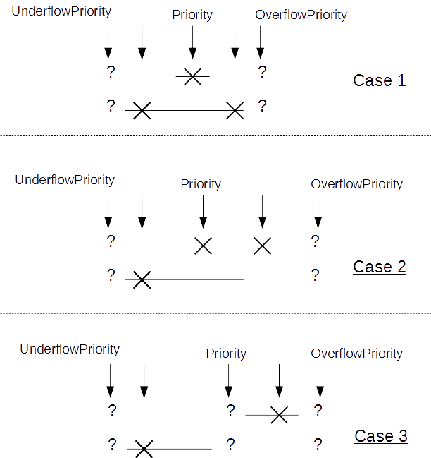
1. One input sample might be hit in both table; (Case 1)

2. One input sample might miss in both table due to overflow; (Case1, 2, 3)

3. One input sample might miss in both table due to underflow; (Case 1, 2, 3)

4. One input sample might miss in both table due to one table overflow while the other underflow (Case 3)

For all the cases above, hardware need a way to choose how to get the final output thus we expose programmable registers below to allow software program the priority:

Register Name	Description
Priority	One bit register to indicate which table output should be selected as the final output when both hit or hybrid miss happens (case a, d); 0 means X table is selected; 1 means Y table is selected;
OverflowPriority	One bit register to indicate which table output should be selected as final output when overflow for both table happens. (case b) 0 means X table is selected; 1 means Y table is selected;
UnderflowPriority	One bit register to indicate which table output should be selected as final output when underflow for both table happens (case c) 0 means X table is selected; 1 means Y table is selected;

LUT Statistics

When one hardware layer completes, hardware will report statistics below to help software understand whether the LUT table is reasonably programmed.

Statistic register	Description
XHitNum	Number of samples hit on X only
YHitNum	Number of samples hit on Y only
UnderflowNum	Number of samples underflow for both X and Y table
OverflowNum	Number of samples overflow for both X and Y table
PriorityNum	Number of samples both hit on X/Y table or Hybrid miss on X/Y table (Actually, this counter has 2 different meanings which corresponding to a and d case in above section, but since they’re mutual exclusive, we just use one register for them. Software is able to distinguish the different meanings since it knows each LUT coverage)

For each register group, we have dedicated statistic registers above, those counters will be available for read when one hardware completes (by set the producer pointer to this register group). Those statistics won’t be erased until the corresponding register group is enabled (op_en be set)